Market Regime Detection: How Our Desk Classifies Bull, Bear, and Sideways
Market regime detection in plain terms: the two rules our desk runs on SPY and QQQ, what happens when they disagree, and what neither can tell you.
Market regime detection sorts price history into a small number of named states — bull, bear, or sideways — so every other decision can be filtered through the state the market is actually in. This desk runs two rules side by side: a deterministic moving-average-and-volatility test, and a three-state Markov model that infers the state from the return distribution itself.
The worked example, first
Here is exactly what the default rule produced on 2026-08-23 from closes through 2026-08-21, recorded in the week-34 desk log. Every input is arithmetic on two years of daily closes — 501 bars, pulled from Yahoo Finance via yfinance and computed in code rather than read off a chart.
| SPY | QQQ | |
|---|---|---|
| Close (2026-08-21) | 765.72 | 713.44 |
| 200-day SMA | 707.54 | 652.78 |
| 50-day SMA | 751.75 | 713.44 |
| Price vs 200-day | +8.22% | +9.29% |
| 50-day vs 200-day | +6.25% | +9.29% |
| 20-day realized vol (annualized) | 13.15% | 22.32% |
| 1-year median of that vol | 12.54% | 17.73% |
| Vol state | elevated (1.05x) | elevated (1.26x) |
| Classification | Bull | Bull |
In plain text: on the 2026-08-21 close, SPY sat 8.22% above its 200-day average and QQQ sat 9.29% above its own, both with the 50-day average above the 200-day, so both classified as Bull under this desk’s rule. The volatility column is where they diverge: SPY’s 20-day reading was barely above its own one-year median while the Nasdaq-100 proxy ran at 1.26 times its median. Same two words, materially different day-to-day behaviour — which is why the ratio is published and not just the label.
What a regime read is — and what it is not
A regime label describes where price has been relative to its own history. It is not a forecast. When this desk writes “SPY classifies as Bull,” the claim is narrow: on the most recent close, price sat above its 200-day average and the 50-day average sat above the 200-day. Nothing in that says where the next 20 sessions go.
The distinction matters because regime labels are easy to over-read. A trend classification is a summary statistic with a lag built in, and it will be wrong at exactly the moments it would be most valuable — the turns. What it does reliably is stop a chart from being read in isolation.
The three computed inputs
Price versus the 200-day simple moving average. The average of the last 200 closes, with the gap recorded as a percentage rather than a yes/no. An asset 0.3% above its 200-day line and one 9% above it are in materially different situations even though both pass the same test.
The 50-day average versus the 200-day average. This compares a shorter trend to a longer one. It sits alongside the first test because price is noisy and a single close can clear a long average on a one-day move; an average-versus-average comparison cannot.
Twenty-day realized volatility against its own one-year median. An annualized standard deviation of daily returns over a 20-session window, always divided by the trailing one-year median of that same measure for that same asset. The cut is the median itself: a ratio above 1.00x prints elevated, at or below prints normal. Our own passes make the boundary visible — 1.01x printed elevated in week 35 with the log noting it was “effectively at the median,” 0.91x and 0.83x printed normal, and 0.65x/0.76x in week 36 were not flagged at all. The ratio is always published next to the word, because 1.05x and 1.26x carry the same label and describe very different weeks. One convention remains unpublished: the return basis and annualization factor behind the volatility figure itself, which is ours to close.
This input is kept separate from the trend classification on purpose — volatility state and trend direction are different questions, and collapsing them into one label hides more than it reveals.
The classification rule
- Bull — price above the 200-day SMA and the 50-day SMA above the 200-day SMA.
- Bear — price below the 200-day SMA and the 50-day SMA below the 200-day SMA.
- Sideways — anything else, meaning the two tests disagree.
# Illustrative: the classification rule and the volatility cut, exactly as specified above.
def classify(closes, vol_20d, vol_1y_median):   # closes = daily closes, newest last
    sma200 = sum(closes[-200:]) / 200
    sma50  = sum(closes[-50:]) / 50
    if closes[-1] > sma200 and sma50 > sma200:  trend = "Bull"
    elif closes[-1] < sma200 and sma50 < sma200: trend = "Bear"
    else:                                        trend = "Sideways"
    ratio = vol_20d / vol_1y_median
    return trend, ("elevated" if ratio > 1.0 else "normal"), round(ratio, 2)

classify(spy_closes, 13.15, 12.54)              # -> ('Bull', 'elevated', 1.05)
The volatility ratio is attached as a separate note. A market can be in a bull classification and an elevated-volatility state at the same time, and saying so is more useful than forcing one word to carry both facts.
One artifact from that same run is worth showing because it is the kind of thing a mechanical method will hand you: QQQ’s close of 713.44 and its 50-day average of 713.4416 round to the same figure — at full precision the close sat about 0.16 cents below the average. That is a rounding coincidence, not a signal. The desk checked the underlying series and found 60 distinct closes in the last 60 bars, confirming it was not a stale-data artifact. A method that generates numbers automatically also generates occasional numbers that look meaningful and are not, and the discipline is to check them rather than narrate them — the same rule that governs a trading journal entry.
When a second method disagrees
Rule-based moving-average classification is not the only approach. Regime-switching statistical models infer states from the return distribution itself rather than from fixed price thresholds. For the week-34 pass the desk ran a three-state Markov chain as the primary method and kept the SMA rule as a cross-check. The Markov run fit ten years of daily closes — 2,513 rows, 2016-08-23 to 2026-08-21 — labelling each 20-day window Bull or Bear only when its return cleared ±5%, and Sideways otherwise.
The two methods returned different labels. The Markov model put both SPY and QQQ in Sideways as of the 2026-08-21 close. The SMA rule called both Bull. Both were run on the same closes, and neither is broken.
| Markov output, 2026-08-21 close | SPY | QQQ |
|---|---|---|
| Current state | Sideways | Sideways |
| P(next = Bear) | 2.13% | 3.58% |
| P(next = Sideways) | 93.09% | 89.07% |
| P(next = Bull) | 4.78% | 7.35% |
| Directional tilt (bull − bear probability) | +0.026 | +0.038 |
| Long-run share: Bear / Sideways / Bull | 7.5% / 79.0% / 13.5% | 11.1% / 63.9% / 25.0% |
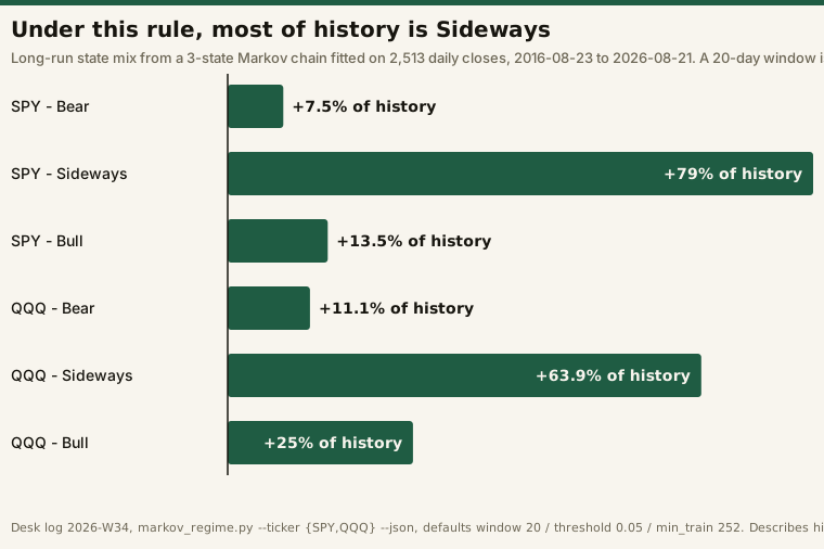
The disagreement is definitional rather than contradictory, and that is the useful part. The SMA rule asks where price sits relative to its own long averages; both ETFs were comfortably above their 200-day lines. The Markov model asks a different question — did the trailing 20-day window move more than ±5%? Most windows do not, and the long-run mix reflects that. A slow grind higher registers as Sideways under one definition and Bull under the other. The tilt figures sit on that model’s own −1 to +1 scale, so +0.026 and +0.038 are very close to neutral.
What we hold of the transition matrix, and what we do not
The chain’s stickiness is the thing the SMA rule cannot tell you at all. Our log records the persistence diagonal for both tickers and the full row for the state they were actually in — and nothing else:
| Transition probability | SPY | QQQ |
|---|---|---|
| Bear → Bear | 0.775 | 0.794 |
| Bear → Sideways / Bull | not recorded | not recorded |
| Sideways → Bear | 0.0213 | 0.0358 |
| Sideways → Sideways | 0.931 | 0.891 |
| Sideways → Bull | 0.0478 | 0.0735 |
| Bull → Bull | 0.721 | 0.812 |
| Bull → Sideways / Bear | not recorded | not recorded |
Four of the nine cells per ticker are not in our record, so we are not printing a complete 3×3 matrix and will not interpolate one. What the recorded cells say is that every state is sticky, and Sideways most of all: given a Sideways reading, the chain puts 93.09% on SPY still being Sideways at the next step. That is a property of a 20-day ±5% labelling rule applied to an index, not a market insight.
Why the walk-forward numbers are not on this page
That Markov run also produced a no-lookahead walk-forward backtest, and it is deliberately absent here. Our log records its Sharpe ratios, maximum drawdowns and trade count — but it does not record the rule that turns a state label into a trade: whether the simulated position is long when the state is Bull, long whenever the tilt is positive, or something else. A performance statistic without the rule that generated it is not checkable — the same standard behind every check we run before a rule trades a dollar — and this page’s whole argument is that a regime number is worthless without its definition. Publishing our own figures while breaking that rule would be the one thing this page cannot afford to do. When the trade rule is written down in the log alongside the period and the parameters, the numbers get published with it.
What the walk-forward check does establish, without any figures at all, is the point of this page: a regime model is a context filter, not a trading system.
Where these methods are weak
They lag. Moving averages are backward-looking by construction, and a 20-day return window is too. Neither flags a regime change until enough closes have accumulated to move it.
Threshold rules whipsaw. When price oscillates around the 200-day line, the SMA classification can flip between Bull and Sideways repeatedly without anything meaningful having changed — which is why the percentage gap is recorded alongside the label.
The label depends entirely on the definition. Week 34 is the plain demonstration: two defensible methods, same data, different words. Anyone reporting a regime without publishing the rule behind it is reporting an opinion.
Why we publish the method before the reads
A regime read is only checkable if the rule that produced it is public, which is the same commitment behind our tool-trial protocol and behind our options-backtest fill comparison, where naming the fill convention is what makes the result interpretable at all. Publishing the inputs, thresholds and data source means the classification we post can be recomputed from the same closes and either confirmed or contradicted — and it makes visible the places where we are not there yet. The two trend tests and the volatility cut now reconcile fully. The annualization convention behind the volatility figure and the trade rule behind the walk-forward backtest do not, and both are named above rather than buried. The label is not the deliverable; the auditability is.
None of the above is a recommendation to buy or sell anything, and a regime classification is not a prediction of future prices. It is a description of the past, kept deliberately simple so that its errors are visible instead of buried.
Frequently asked questions
What does “market regime” mean?
A regime is a named state of the market — most commonly bull, bear, or sideways — summarizing prevailing trend and volatility conditions over a period. Frameworks define the boundaries differently, so the label only has meaning alongside the rule that produced it.
Does a bull classification mean prices will keep rising?
No. The classification states that price is above its long-term average and that the shorter average is above the longer one. Both statements describe history. Neither implies anything about subsequent returns.
When is volatility “elevated”?
On this desk, when the 20-day annualized realized volatility is above the trailing one-year median of that same measure — a ratio above 1.00x. The ratio is always published next to the word, because 1.01x and 1.26x both print elevated and mean very different things.
Which method should be trusted when two regime models disagree?
Neither, in the sense of picking a winner. A disagreement between a price-threshold rule and a return-distribution model is itself information — typically a slow drift that clears one test and not the other. Read both labels next to their definitions rather than collapsing them into one word.
How often should a regime read be run?
The inputs move slowly by design, so daily recomputation on averages this long mostly produces noise. What matters more than cadence is logging the date of the closes used, so any read can be reproduced against the exact series behind it.