Trend Following Diversifier Backtest: The Return and the Low Correlation Were in Different Variants

In our backtest of a trend-following diversifier, no variant was both profitable and uncorrelated. The tradeable long-or-cash version earned 2.6% a year but had a +0.49 correlation to our QLD trend strategy. The long-or-short version had a +0.09 correlation but lost 1.8% a year. And when we blended the sleeve in, the lower drawdown came from dilution, not protection (backtest simulation — not live results, not a prediction, not advice).

Every figure on this page is a backtest simulation — not live results, not a prediction, not advice. The figures come from a desk research record (mf_trend_results.md, run 2026-07-29). The window is 2008–2026, and the rule is a 200-day trend filter on seven ETFs at equal weight with 3 bps of cost per side.

The rule being tested

The sleeve is a simple multi-asset trend rule built from ETFs. The parameters, as the record states them:

Parameter	Setting
Universe	SPY, EEM, TLT, IEF, GLD, DBC, VNQ
Signal	200-day trend
Weighting	1/N (equal weight across the seven)
Costs	3 bps per side
Window	2008–2026
Comparison	Correlation to a QLD trend strategy

Two variants were run. Long-or-cash holds an ETF while it’s in an uptrend and sits in cash otherwise. That’s the variant you can actually trade with ordinary ETFs. Long-or-short goes short instead of to cash when the trend is down. The record labels it “theoretical”, so treat it as a reference point, not a tradeable result.

Here’s the mechanism as code. It’s a simplified illustration, not the desk’s research code. It assumes “in trend” means the close is above its 200-day average, which the record doesn’t spell out:

# Illustrative only: 200-day trend sleeve, 1/N, 3 bps per side.
import pandas as pd

def trend_sleeve(closes: pd.DataFrame, short: bool = False, cost_bps: float = 3) -> pd.Series:
    rets = closes.pct_change()
    up = closes > closes.rolling(200).mean()
    pos = up.astype(float) - ((~up).astype(float) if short else 0.0)  # +1 / 0, or +1 / -1
    pos = pos.shift(1)                                     # trade on yesterday's signal
    w = pos / closes.shape[1]                              # 1/N across the universe
    turnover = w.diff().abs().sum(axis=1)
    return (w * rets).sum(axis=1) - turnover * cost_bps / 10_000

# Diversification is then a single number:
# trend_sleeve(etfs).corr(qld_book_returns)

The short flag is the whole difference between the two variants. Everything else is identical.

The result: return in one variant, uncorrelation in the other

The record’s table, verbatim:

variant	CAGR	Sharpe	maxDD	corr to QLD	2020	2022
long-or-cash (tradeable)	2.6%	0.45	−13.1%	+0.49	+6.9%	−5.3%
long-or-short (theoretical)	−1.8%	−0.06	−38.2%	+0.09	+0.4%	+4.2%

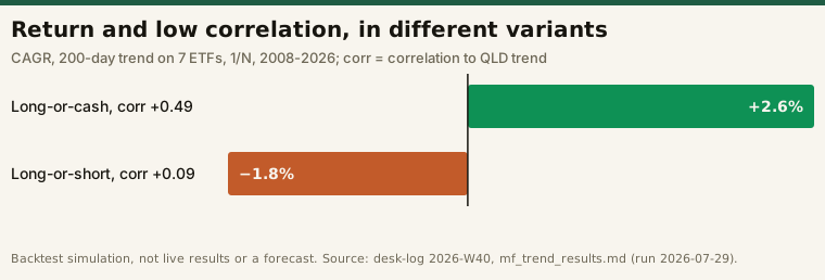
The two properties people want from a diversifier ended up in different rows.

The tradeable variant earned, but it didn’t diversify. The record’s explanation: “SPY + EEM are equity trend, which overlaps QLD (also equity trend). A sleeve that’s ⅓ equity-trend can’t diversify an equity-trend book.” When equities trend down, both the strategy and the sleeve’s equity legs step aside together. When equities trend up, both hold them. A +0.49 correlation is what that overlap looks like as a number.

The uncorrelated variant diversified, but it lost money. Long-or-short shows what the record calls “the classic MF crisis signature”: +4.2% in 2022, a year in which the long-or-cash variant lost 5.3%. Its correlation to the strategy was close to zero. But over the full window it returned −1.8% a year, with a −38.2% drawdown, nearly three times the long-or-cash variant’s. The record’s diagnosis: “The theoretical short leg got run over in the 2010s (shorting false-downtrends in a relentless bull), erasing the crisis wins.”

So the short leg is where the uncorrelation came from, and it’s also where the money was lost. In this window you couldn’t keep one and drop the other.

The blend test: lower drawdown, no better floor

The second stage asked the practical question: what happens to the strategy when you blend the sleeve in? The record reports three steps of that blend. The excerpt doesn’t give the weights at each step, so we don’t either. Verbatim:

The blend cuts drawdown (−40% → −31% → −24%) — but that’s diversification-by-dilution, not floor-lifting: the worst-5yr floor does NOT improve (4.2% → 4.1% → 3.5%, flat-to-lower), time-underwater barely moves (459 → 448d), and median return drops sharply (23% → 14%).

Laid out as a table, using the record’s own labels (the record doesn’t define the measurement period behind “worst-5yr floor” or “median return”, or say whether time-underwater is the longest spell, so we don’t either; the time-underwater and median figures are given only at the ends of the range):

Blend step, as reported	Drawdown	Worst-5yr floor	Time-underwater	Median return
Step 1	−40%	4.2%	459 days	23%
Step 2	−31%	4.1%	—	—
Step 3	−24%	3.5%	448 days	14%

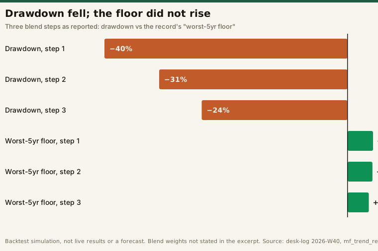
Judged on drawdown alone, the blend worked: drawdown shrank by 16 points across the steps. Every other column says the improvement was mechanical. Swapping part of a volatile strategy for a low-volatility sleeve shrinks the drawdown in proportion, whether or not the sleeve does anything useful in a crash. A sleeve that truly protected the strategy would lift the worst five-year stretch and shorten the time spent underwater. Neither happened. The worst 5-year floor went flat-to-lower, time underwater moved by 11 days, and the median return fell by 9 points.

That’s the distinction the record draws between “diversification-by-dilution” and “floor-lifting”. Only the second one is worth paying for.

A second sleeve, the same answer

This wasn’t a one-off. An earlier desk study tested a different kind of sleeve: an RSI(2) mean-reversion rule on the 11 SPDR sector ETFs, 2016-01 to 2026-07, 3 bps per side, with each ETF from its own inception. It had a 0.385 correlation to QLD, which is what “diversifier” is supposed to mean. Then an 80/20 QLD-plus-sleeve blend over 2016–2026, verbatim from the record:

metric	QLD-alone	80/20 blend
worst rolling 5yr CAGR	15.5%	13.2% (lower)
median rolling 5yr CAGR	32.8%	26.8% (lower)
max time-underwater	375d	373d (unchanged)

Again, backtest simulation — not live results, not a prediction, not advice. The record’s conclusion: “A low-return, low-corr, low-DD sleeve can’t improve a 20%-CAGR book on a floor metric — you’d need the sleeve to actually earn during QLD’s bad windows, and it doesn’t earn enough.” This is a different study from the single-instrument QQQ RSI(2) sleeve whose out-of-sample check is covered in backtesting mistakes that only real data reveals; the sector version broadens the universe to 11 ETFs.

Two different sleeves and two different windows gave the same lesson. Low correlation describes the shape of two return streams. It says nothing about whether the sleeve earns enough to pay for the room it takes up.

What this backtest can’t tell you

The window leaves out trend following’s strong era. The record’s own caveat: 2008–2026 “excludes the managed-futures strong era of the 1980s–2000s.” A longer history could change the long-or-short result. This test can’t say either way.

It’s one construction. One lookback (200 days), one weighting (1/N), seven ETFs. The result describes this rule, not trend following in general.

Correlation is to one specific strategy. The +0.49 is measured against an equity trend strategy. Against a different portfolio, the same sleeve would show a different correlation, and possibly a different blend result. A different way of cutting a QLD strategy’s drawdown, de-levering to QQQ when volatility spikes, is tested in our QLD volatility de-lever backtest.

The full sequence of checks we run before believing a backtest is in how we validate a strategy.

How to read any diversifier backtest

1. Find the correlation’s counterpart. “Low correlation” has to be measured against something. Check that it’s measured against your own holdings, not a generic index.
2. Check the return and the correlation come from the same variant. A pitch that quotes the long-short version’s correlation and the long-only version’s return is quoting two different strategies.
3. Look at what each leg contributes. If the uncorrelation comes from a short leg, check what that leg did in long bull runs.
4. Judge a blend on its floor, not its drawdown. Ask for the worst rolling multi-year return and time underwater, before and after. A smaller drawdown with a flat floor is dilution.
5. Check the window against the strategy’s history. A diversifier tested only in one kind of market hasn’t shown much about the others.

Frequently asked questions

Does a trend-following sleeve diversify an equity portfolio?

In this backtest, the tradeable long-or-cash version didn’t diversify much: it had a +0.49 correlation to an equity trend strategy, because two of its seven ETFs (SPY and EEM) are equity trend themselves. The long-or-short version had a +0.09 correlation but lost 1.8% a year over 2008–2026. Backtest simulation — not live results, not a prediction, not advice.

Why did the long-or-short version lose money?

According to the desk record, the short leg “got run over in the 2010s”, shorting trends that reversed during a long bull market. That erased gains from crisis years such as 2022, when the variant returned +4.2%. The test window, 2008–2026, also leaves out the 1980s–2000s, an era the record calls managed futures’ strong period.

If blending cuts drawdown, isn’t that diversification?

Not necessarily. In this blend test, drawdown fell from −40% to −24%, but what the desk record calls the “worst-5yr floor” went from 4.2% to 3.5%, time-underwater barely moved (459 to 448 days), and the median return fell from 23% to 14%. That pattern is dilution: a smaller position in the volatile asset, not protection from the new one.

What should a diversifier improve, then?

The floor. A useful diversifier should lift the worst multi-year stretch or shorten the time spent underwater, which means it has to earn money while the main strategy is losing. In both desk blend tests on this page, the floor didn’t improve.

---

This is educational content about research method, not financial advice. No positions, live signals, account values or trading results appear on this page. All figures are historical backtest simulations over the stated periods — not live results, not predictions, not a recommendation.