Leveraged ETF Volatility Filter Backtest: Nearly Free for a Decade, Then 7 Points a Year

In our backtest, a volatility filter that switched from the 2x Nasdaq ETF QLD to the 1x QQQ whenever QLD’s 20-day volatility rose above 35% cut maximum drawdown in both halves of a 20-year test. That makes the drawdown cut look real rather than a fitting artifact. The cost wasn’t stable, though. Over the full sample it averaged −4.0 percentage points of CAGR. That average combined about −1.4 points a year in 2006–2015 with −7.0 points a year in 2016–2026.

So the robustness check passed, and it also showed that the headline cost was an average of two very different regimes. This page shows the numbers and how the check was run.

Every figure below is a backtest simulation — not live results, not a prediction, not advice. The figures come from a desk research record: real adjusted QQQ and QLD daily data from 21 June 2006 to 30 June 2026, study run on 1 July 2026, with the split-sample check run by run_qld_oos.py. They describe what a rule did over those dates and say nothing about what it will do.

The rule being tested

The overlay is one line of logic layered on the study’s baseline QLD strategy. That baseline is not buy-and-hold: the desk’s QLD studies use a trend rule on QLD as their base (one study’s table labels it “plain QLD trend”), and a separate desk study over the same 2006–2026 window put QLD buy-and-hold at a −84% maximum drawdown, far deeper than the −49.8% baseline below (backtest simulation — not live results, not a prediction, not advice).

• Signal: QLD’s trailing 20-day volatility.
• Threshold: 35%, with 30% and 45% tested alongside.
• Action: while volatility is above the threshold, hold QQQ (1x) instead of QLD (2x). Return to QLD when it falls back below.
• Comparison: the same baseline without the overlay, on the same data and dates.

Here’s the mechanism as code. This is a simplified illustration, not the desk’s research code. The annualisation by √252 is the usual convention and is assumed here, and the baseline’s trend rule is left out:

# Illustrative only: the de-lever overlay, without the baseline's trend logic.
import numpy as np
import pandas as pd

def delever_returns(qld: pd.Series, qqq: pd.Series, threshold: float = 0.35) -> pd.Series:
    r_qld, r_qqq = qld.pct_change(), qqq.pct_change()
    vol20 = r_qld.rolling(20).std() * np.sqrt(252)   # annualised 20-day realised vol
    high_vol = (vol20 > threshold).shift(1, fill_value=False)  # decide on yesterday's close
    return r_qqq.where(high_vol, r_qld)              # 1x in high vol, 2x otherwise

def cagr(r: pd.Series) -> float:
    years = len(r.dropna()) / 252
    return (1 + r.fillna(0)).prod() ** (1 / years) - 1

def max_dd(r: pd.Series) -> float:
    eq = (1 + r.fillna(0)).cumprod()
    return (eq / eq.cummax() - 1).min()

The shift(1) matters. A rule that reads today’s volatility and trades at today’s close has used information it couldn’t have had in time to act on.

The full-sample result

Over the whole 2006–2026 window, the 35% threshold looked like a clean trade-off. Here’s the record’s headline, laid out as a table:

Full sample, 2006-06-21 to 2026-06-30	Baseline	De-lever at vol > 35%
Max drawdown	−49.8%	−35.1%
CAGR change	(baseline)	−4.0pp
Sharpe ratio	0.79	0.81

That’s 14.7 points less drawdown for 4 points a year, with a slightly better Sharpe ratio. Read on its own, it looks like a fixed price for a fixed amount of protection. The split-sample check shows that it isn’t.

The split-sample check

The check asks one question: does de-levering cut drawdown in each half of the history when the halves are tested separately? If the effect only appeared in one half, the full-sample result would just be that one episode.

The two halves are very different markets. 2006–2015 contains the global financial crisis. 2016–2026 is mostly a strong bull market with sharp V-shaped recoveries. The record’s table, verbatim:

period	base maxDD	vol>0.30	vol>0.35	vol>0.45
IS 2006-2015 (GFC era)	−49.8%	−26.3% (−1.1pp CAGR)	−31.4% (−1.4pp)	−47.9% (+1.0pp)
OOS 2016-2026 (bull)	−40.2%	−30.2% (−10.0pp CAGR)	−28.3% (−7.0pp)	−30.5% (−3.6pp)

Each cell is the maximum drawdown at that threshold, with the change in CAGR against the baseline in brackets. “IS” and “OOS” are the record’s labels for the two halves. This is a split-sample check, not a walk-forward test: the threshold was not re-fitted as the window moved.

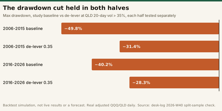
The core question passed. At the 35% threshold, drawdown fell in both halves: −49.8% to −31.4% in the GFC decade, −40.2% to −28.3% in the bull decade. The record calls the threshold “a smooth monotonic dial (lower = more protection = more CAGR cost), no lonely spike.” A parameter that only works at one exact value is usually fitted to noise. One that changes smoothly across a range is at least a candidate for a real effect.

What the average was hiding

The same table shows something the pass/fail question doesn’t. The cost of that protection depended on which decade you were in.

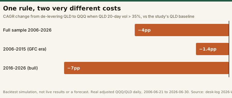
• 2006–2015: de-levering at 35% cost 1.4 points of CAGR. The record says it was “nearly free” and “raises Sharpe — you skip losses.” Holding 1x through a crash-heavy decade mostly meant missing declines.
• 2016–2026: the same rule cost 7.0 points of CAGR, from 29.5% to 22.5%. The record’s explanation: “you’re at 1× during the sharp V-recoveries (2018/2020/2022) where 2× would have ripped.” Volatility stays high for a while after a sharp drop. So a volatility trigger keeps you at half leverage through the rebound, which is exactly when 2x pays most.

The full-sample −4.0 points describes neither decade. Someone who sized their expectations from the headline would have found the filter much cheaper than expected through the first decade and much more expensive through the second. The per-decade figures above are a historical record. Neither is an estimate of what the filter will cost next.

The dial behaves differently by decade too. At 30%, the bull-decade cost rises to 10.0 points while the GFC-decade cost stays at 1.1. At 45%, the GFC decade barely gets any drawdown cut (−49.8% to −47.9%), while the bull decade still gets a sizeable one (−40.2% to −30.5%) for 3.6 points. No single threshold has the same trade-off in both regimes.

What this check can’t tell you

Three limits apply to every number on this page.

QLD only exists from 2006. A related desk study on the same instruments notes that the window “can’t test a dot-com-magnitude Nasdaq grind (2000–02), where a 2× would fare worse than shown.” Every worst case here is bounded by the fund’s listing date, not by how bad markets can get.

Two halves is a small sample of regimes. Splitting 20 years into two gives one crash decade and one bull decade. That’s enough to show the cost is regime-dependent. It isn’t enough to say how the cost is distributed across regimes in general.

The threshold was chosen on the full sample. The split-sample check tests whether the effect appears in both halves. It doesn’t remove the fact that 35% was picked while looking at all 20 years. That’s why the result counts as surviving a check, not as validated. Blending in a diversifying sleeve is another way to shrink a QLD strategy’s drawdown; in our trend-following diversifier backtest, the smaller drawdown turned out to be dilution, not protection. The full sequence of checks we run before believing a backtest is in how we validate a strategy.

One data note: QLD’s history needed cleaning before any of this was possible, because our data source padded rows before the fund existed. That story is told once, in backtesting mistakes that only real data reveals.

How to read any “volatility filter” backtest

1. Find the baseline. A drawdown cut is only meaningful against a stated comparison. Here it’s a QLD trend rule, not buy-and-hold, so these figures don’t describe holding QLD outright.
2. Ask for the split. A single full-sample cost figure can average a cheap decade with an expensive one. Request the same table for at least two different regimes.
3. Check the threshold sweep. Look for a smooth dial, not one spike, and check whether the dial behaves the same way in each regime.
4. Check the timing. The signal has to be computed from data available before the trade.
5. Check the start date against the instrument’s history. A leveraged ETF’s backtest can’t include crashes that happened before it launched.

Frequently asked questions

Does a volatility filter reduce drawdowns on a leveraged ETF?

In this backtest it did. De-levering from QLD to QQQ when QLD’s 20-day volatility exceeded 35% cut maximum drawdown in both 2006–2015 (−49.8% to −31.4%) and 2016–2026 (−40.2% to −28.3%), against the study’s QLD trend baseline. Backtest simulation — not live results, not a prediction, not advice.

How much return did de-levering cost?

It depended on the period. Over 2006–2026 the cost averaged 4.0 points of CAGR at the 35% threshold. In 2006–2015 it was 1.4 points. In 2016–2026 it was 7.0 points (29.5% to 22.5%), mostly because the rule held 1x through sharp recoveries. These are historical simulation figures for the stated periods, not an expected cost.

Is a split-sample check the same as walk-forward testing?

No. A split-sample check tests a fixed rule on two separate stretches of history. Walk-forward testing re-fits the rule on a rolling window and evaluates each fit on the data that follows it. This study ran the split-sample version only.

Why is the baseline drawdown only −49.8% if QLD is a 2x ETF?

Because the baseline isn’t buy-and-hold. It’s a trend rule on QLD, the base the desk’s QLD studies share. For comparison, a separate desk study over the same 2006–2026 window measured QLD buy-and-hold at a −84% maximum drawdown. Backtest simulation — not live results, not a prediction, not advice.

---

This is educational content about research method, not financial advice. No positions, live signals, account values or trading results appear on this page. All figures are historical backtest simulations over the stated periods — not live results, not predictions, not a recommendation.